Basic Video Processing

Hello and welcome to the final blog post. It’s been quite an adventure, and definitely a learning experience for me. I hope this blog will also be helpful to the few eyes that read it haha!

See how happy we are that we took this class! From Left to Right: Ron Aves, Myself, and Jesli Santiago

I’d also make a quick detour and thank my professor in this class, Dr. Maricor Soriano, for all the wisdom and knowledge she has passed on to our class, and who is probably our highest authority when it comes to image and video processing here in our university, especially when it is related to scientific research. If you have a chance, feel free to check out her own blog for more information on image and video processing. (http://a-little-learning.blogspot.com).

 

Now, back to basic video processing. As we all know, a video is just a series of images taken over a certain time frame. For example, the video recorder we use in class takes 60 frames per second. That means in one second, it would have taken 60 images in quick succession that, when viewed in the camera or in the computer, looks exactly the same as what we would see with our eyes if we didn’t have the camera.

 

We can do a lot more with videos than that we can do with pictures. For example, instead of just taking one scene from an event, we can record the event and see all that when on during that event again and again and again and again. But as with pictures, sometimes what we want can’t be immediately seen or understood just by seeing the raw video. What if we want to track an object? Or a person for that matter? What if we wanted to study how organized is the road system in a certain city? For that, we need video processing, and for our purposes, basic video processing just means applying image processing to each of the frames of the video.

 

For this lesson, I teamed up with two of my classmates to conduct an experiment. We wanted to verify the value for gravity from the motion of an object moving down an inclined plane.

Figure 1. An object rolling down an inclined plane [1].

Why? By doing so, we can show that video processing can be used to track an object, and be able to calculate variables from the video alone. Think of how Tony Stark made Jarvis so intelligent and his Iron Man suit so capable of multiple enemies!

Come on, who doesn’t want repuslor beams in their gauntlets? [2] 

But remember that we’ll only be doing basic video processing here. A lot of what’s in our videos will be filtered out and cropped so that we can track our object. So without further ado, let’s begin!

 

First, some of our materials and methodology for the experiment.

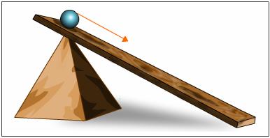
We had a video camera (60 fps) positioned right above the plank similar to the setup in Figure 1. Now, to minimize the effects of a rolling object on our value for gravity, we chose to only have small angles of inclination. To increase the angle, we just added objects to prop our plank. For our object, we had a small metal cylinder that rolls down the plank. Then we simply recorded the cylinder from the top of the plank until it arrived at the bottom of the plank.

Figure 2. A snapshot of our setup

In order to be a little more accurate, we recorded the motion for four angles of inclination.

We then converted each video into jpg frames using DVDVideoSoft’s Free Video to JPG Converter (download link is here https://www.dvdvideosoft.com/products/dvd/Free-Video-to-JPG-Converter.htm#.Vl3PhzZem48).

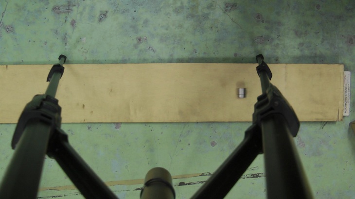
In order to simplify the process, we only took the frames of the cylinder within the legs of the video camera’s stand. Simplifying it further, we crop out the floor, leaving only the portion of the plank where the cylinder rolls.

Next, we use parametric segmentation in order to find the portion of the frames that comprises of the cylinder. (Refer to my previous post on the subject if you’d like to learn more about it). Now, since the cylinder is gray, then in parametric segmentation it will appear like the rest of the image also has color components of the ROI we chose (since white-gray-black appear the same in parametric and nonparametric segmentation). However, the degree of the segmentation will be enough that we can filter the background out using the same step we did to remove the background from a cropped check ( Again, refer to the post on image segmentation. The code looks a bit like I2 = I > a number). Finally, using our knowledge of morphological operations to good use, we use the Open function with a Rectangular Structuring Element to remove the rest of the background, leaving only the cylinder, and then we use the Close function to fill it in just in case some parts of the cylinder were removed by the Open function.

Repeating for each of the frames, we will be able to see the movement of the cylinder as shown below. If you would like to make your own GIFs, I suggest checking out http://gifmaker.me

Figure 3. The movement of the cylinder. From top to bottom, the height increases, hence the cylinder moves the fastest in the bottom GIF.

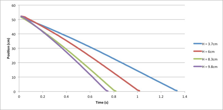
From there, we can get the location of the cylinder and find its position over time. To do so, we make use of areaprops of Matlab and find the centroid of the cylinder to make it easier for us to track. Then we simply tabulate the locations of the cylinder at each frame and display it as a graph. To simplify the data, we assume that the cylinder is only moving along the x, and that the movement along the y (rolling to the left or right of the plank) is negligible in this case and shouldn’t affect our value for g. My groupmate Ron found that the 1 pixel is equal to 0.05 cm in real life, so we use that to convert the location of the cylinder into actual centimeters. Again, to find time, we just need to remember that the video records at 60 frames per second.

Figure 4. Position Versus Time of the cylinder for different heights

In order to get the velocity from this plot, we need to read the array in Matlab, then use the builtin diff() function to get the derivative of x and t, leaving us with the velocity. Again, we can create a plot of the velocity versus time in excel.

Figure 5. Velocity versus time of the cylinder

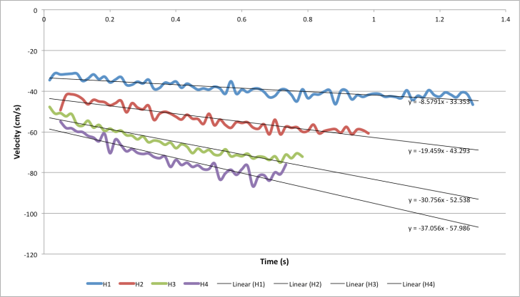
This is an incredibly noisy plot. Don’t mind the negative sign, this is because in our image the cylinder was moving in decreasing pixel locations. If we had more frames to work with or had a better setup where the cylinder moves only along the x-axis, this might look better. But let’s see if we can still use this data to find the acceleration.We can get the slope of the velocity plots and set it as our acceleration. This leaves us with four values of acceleration for each height. We then find the sin(theta) where theta = height/length of plank, which in this case was 109 cm. We have the following plot that corresponds to that:

Figure 6. Acceleration versus Sin(theta)

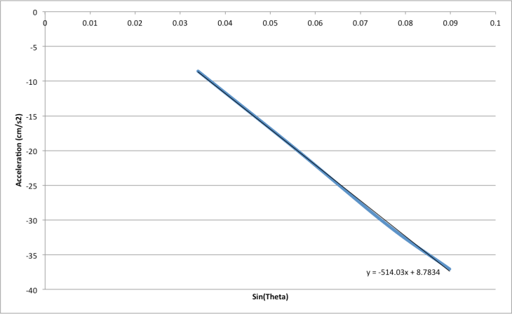
The calculated value for gravity in this case is 514.03 cm/s^2. The theoretical value is -980 cm/s^2. That’s a 47.45% error. Sadly, our result is unacceptable. If we had a setup where the camera’s placement does not interfere with its field of vision, we might have better results. Perhaps you, reader, can do so for your own experiment! At the very least, we are able to find track our object in the video, which is an achievement in itself, and opens a lot of possibilites for such a skill. A possible extension of this would be to show the boundary of the cylinder in the actual video and show it being tracked over the course of the video. You could even extend it for other things such as people or clothing! Who knows?

With that, our final lesson in image and video processing comes to an end. Hopefully, this helps you in your own path in learning image and video processing. Good luck and study hard!

References:

 

1. Image taken from http://www.tutorvista.com/content/science/science-i/force-laws-motion/galileo-observation-origin-newtonian.php
2. Image taken from http://static2.hypable.com/wp-content/uploads/2015/07/iron-man-civil-war-salary-wide.jpg

Code used:

prefix1 = ‘/Users/Jaime/Documents/MATLAB/AP186 Activity 9/AP186_Act9_JPGs/00457’;

prefix2 = ‘/Users/Jaime/Documents/MATLAB/AP186 Activity 9/AP186_Act9_JPGs/00461’;

prefix3 = ‘/Users/Jaime/Documents/MATLAB/AP186 Activity 9/AP186_Act9_JPGs/00467’;

prefix4 = ‘/Users/Jaime/Documents/MATLAB/AP186 Activity 9/AP186_Act9_JPGs/00471’;

 

fnum1 = 121:200;

fnum2 = 096:156;

fnum3 = 098:146;

fnum4 = 126:170;

 

ext = ‘copy.jpg’;

 

%% crop image to only the plank region

base = [prefix1 num2str(121) ext];

Ibase = imread(base);

Ibasecrop = imcrop(Ibase, [330,420, 1050, 150]);

imshow(Ibasecrop)

background = zeros(size(Ibasecrop));

 

%% get RGB, rgb of ROI

I2 = imcrop(Ibasecrop);

I2 = double(I2);

R = I2(:,:,1); G = I2(:,:,2); B = I2(:,:,3);

Int= R + G + B;

Int(find(Int==0))=100000;

 

r = R./ Int; g = G./Int; b = B./Int;

r_mean = mean(mean(r));

r_sigma = std(std(r));

g_mean = mean(mean(g));

g_sigma = std(std(g));

b_mean = mean(mean(b));

b_sigma = std(std(b));

 

 

 

% %% test

% fnum = 121;

% fname = [prefix num2str(fnum(i)) ext];

% I1 = imread(fname);

% Icrop = imcrop(I1, [330,420, 1050, 150]);

%

% Icrop = double(Icrop);

% R2 = Icrop(:,:,1); G2 = Icrop(:,:,2); B2 = Icrop(:,:,3);

% Int2 = R2 + G2 + B2;

% Int2(find(Int2==0))=100000;

% r2 = R2./ Int2; g2 = G2./Int2; b2 = B2./Int2;

%

% probr = (1/(sqrt(2*pi)*r_sigma))*(exp(-(r2-r_mean).^2)/(2*r_sigma^2));

% probg = (1/(sqrt(2*pi)*g_sigma))*(exp(-(g2-g_mean).^2)/(2*g_sigma^2));

% probb = (1/(sqrt(2*pi)*b_sigma))*(exp(-(b2-b_mean).^2)/(2*b_sigma^2));

% jointprob = probr.*probg.*probb;

% imagesc(jointprob)

% colormap(gray)

%

% Itest = jointprob > mean(mean(jointprob))+mean(mean(jointprob))*0.003;

% imagesc(Itest)

% S1 = strel(‘rectangle’, [20 10]);

% Itest2 = imopen(Itest,S1);

% Itest3 = imclose(Itest2,S1);

% imagesc(Itest3)

% s = regionprops(Itest3, ‘centroid’);

% centroids = cat(1, s.Centroid);

% imshow(Itest3)

% hold on

% plot(centroids(:,1),centroids(:,2), ‘b*’);

% hold off

 

%% run for all images of chosen video

data = cell(length(fnum1),1);

for i= 1:length(fnum1)

fname = [prefix1 num2str(fnum1(i)) ext];

I1 = imread(fname);

Icrop = imcrop(I1, [330,420, 1050, 150]);

Icrop = double(Icrop);

R2 = Icrop(:,:,1); G2 = Icrop(:,:,2); B2 = Icrop(:,:,3);

Int2 = R2 + G2 + B2;

Int2(find(Int2==0))=100000;

r2 = R2./ Int2; g2 = G2./Int2; b2 = B2./Int2;

 

probr = (1/(sqrt(2*pi)*r_sigma))*(exp(-(r2-r_mean).^2)/(2*r_sigma^2));

probg = (1/(sqrt(2*pi)*g_sigma))*(exp(-(g2-g_mean).^2)/(2*g_sigma^2));

probb = (1/(sqrt(2*pi)*b_sigma))*(exp(-(b2-b_mean).^2)/(2*b_sigma^2));

jointprob = probr.*probg.*probb;

Itest = jointprob > mean(mean(jointprob))+mean(mean(jointprob))*0.003;

S1 = strel(‘rectangle’, [20 10]);

Itest2 = imopen(Itest,S1);

Itest3 = imclose(Itest2,S1);

%     jpgname = [‘video1’ num2str(fnum1(i)) ‘.jpg’];

%     imwrite(Itest3, jpgname);

s = regionprops(Itest3, ‘centroid’);

centroids = cat(1, s.Centroid);

imshow(background)

hold on

plot(centroids(:,1),centroids(:,2), ‘b*’);

hold off

%     prefixfinal = ‘/Users/Jaime/Documents/MATLAB/AP186 Activity 9/00457’;

%     extfinal = ‘.jpg’;

data{i} = centroids;

%     final = [prefixfinal num2str(fnum(i)) extfinal];

%     imwrite(jointprob, final)

end

xlswrite(‘data1.xls’,data)

% figure(2);

% imagesc(imrotate(hist,90))

% colormap(gray)

%% Read the data and produce the velocity plot

d1 = csvread(‘data4.csv’);

X = d1(:,1);

Xcm = X.*0.05;

num = 1:length(X);

t = num./60;

% plot(t,Xcm)

 

% p = polyfit(Xcm,t’,2);

% test = polyval(p,Xcm);

% figure

% plot(t,Xcm,’o’)

% hold on

% plot(test,Xcm,’r–‘)

% hold off

 

v = diff(Xcm’)./diff(t);

num2 = 1:length(v);

t2 = num2./60;

plot(t2, v)

 

xlswrite(‘v4.xls’,v);